The Semi-Symmetric Metric Connection – Part II

Mathematical Preliminaries

In the previous post in this series, I gave the rationale for undertaking this extended (re-)examination of the geometry of the semi-symmetric metric connection (SSMC): essentially, it represents (to my mind) the most ultra-minimalist extension to General Relativity (GR) at all possible – or so I thought back in the early 1990s – given that it introduces precisely one new object – a vector field – as part of the connection.

In gauge field theories the “connection” carries the gauge field, while the “curvature” corresponds to the field strength, a view that was argued in a book by Göckeler and Schücker (1989), which I had also been reading at that time. Since electromagnetism is often introduced as the archetypal gauge field in mathematical treatments of differential geometry (such as that by Göckeler & Schücker), it seemed to make intuitive sense to me that introducing electromagnetism into an extension of GR intended to model electromagnetism by way of a geometrical object might require it to enter by way of the connection, rather than as an additional field just lying around in spacetime, as it is in Einstein-Maxwell Theory (EMT). Hence, in this view, the SSMC is an obvious candidate.

In what follows, I will establish some basic definitions for some mathematical operations that will be required in the next post (Part III) where we will examine the geometry of the SSMC as a precursor to seeking field equations that may be implicitly contained in the geometry. I will work using the component notation (as opposed to the more elegant component-free form) for tensors, as well as working within a co-ordinate frame (as opposed to non-coordinate frames) which simplifies the number of symbols used.

As noted previously in Part I, I do not intend to follow the standard pathway for finding field equations from a formal mathematical “variational procedure” (a standard approach to classical field theories), which is a very common way that GR is sometimes introduced and developed in contemporary accounts and in many texts. (There are problems with this approach anyway, as it turns out, which I’ll talk about in Part IV, on searching for field equations.)

Rather, I wish to follow and perhaps generalise the original pathway Einstein himself followed when working out GR, which was to look for candidate geometrical objects guided by considerations of physics. It was only after the field equations were written down that a variational approach showed that the field equations so postulated were “compatible”. In 1917 Einstein wrote in a letter to Felix Klein (cited in Pais 1982, p.325):

It does seem to me that you highly overrate the value of formal points of view. These may be valuable when an already found [his italics] truth needs to be formulated in a final form, but fail almost always as heuristic aids.

As Pais then goes on to note, this is indeed striking when compared to how Einstein later searched for a unified field theory based on generalising the formal mathematical variational procedure which can be used to derive the field equations of GR – in effect, ignoring his own advice to Klein. As I delved through the derivations of various versions of non-symmetric forms of Einstein’s unified field theory (EUFT) from 1925 to 1955 during my doctoral work, the contrast between his being guided by considerations of physics in GR and by a desire for formal simplicity in EUFT was indeed quite marked. Pais observes (p.325) that, back then in 1917, Einstein still “knew with unerring instinct how to select complexes from nature to guide his scientific steps.” One could do worse, then (I think), than to seek to emulate the “unerring instinct” of the Einstein of 1917 and to forego – to the degree possible – any over-reliance on “formal points of view” and, instead, to have considerations of physics front-of-mind and center-stage.

As Pais also notes on that page, Einstein’s last act while dying in hospital was to work on the most recent pages of calculations on his unified field theory, after which he collected up his notes, laid down his pen, and went to sleep. He never woke up. This is all the more remarkable since he had said to his collaborator Infeld (1942, p.234) some two decades earlier:

Life is an exciting show. I enjoy it. It is wonderful. But if I knew that I should have to die in three hours it would impress me very little. I should think how best to use the last three hours, then quietly order my papers and lie peacefully down.

This is one of the reasons I found it so enormously compelling working on Einstein’s attempts at a unified field theory – it was literally the last thing he worked on during his amazingly productive life of doing fundamental and revolutionary physics. The overall tone of this little planet in the vast cosmos was immeasurably raised for his having lived here at all, and may be the one genuine claim to fame we have in the universe (as the cartoon at the top of this post suggests, published the day after his death in 1955). He pursued that quest for a unified theory right to the very end…

So, let us now return to that quest, albeit via a much simpler and much less formal pathway than he followed, to see if we might be able to make some headway towards a geometrically-unified account of gravity and electromagnetism that is based on what I think is the simplest step at all possible beyond the elegantly beautiful simplicity of GR.

In the following, I will largely follow the index-placement conventions of Schouten (1954), since this affords the easiest manner of comparison with his analysis. His discussion is contained in Chap. III (commencing p.121), but which I shall greatly abridge, leaving aside all the detailed definitions of different spaces, as well as changing his notations in a couple of places later where I think it is more useful or intuitive.

In a general (curved) space, it is necessary to introduce something called a connection (Schouten renders it as connexion) $\mathbf{\Gamma}$ which, in the component notation, is usually denoted $\Gamma^\alpha_{\mu\nu}$ . It is important, among other things, for defining differences in the values of functions at “nearby” points, since you need some sense of what “nearby” actually means in order to be able to do this. It is not a tensor, but it does help to define (see below) so-called covariant derivatives of tensors, which are themselves also tensors, as well as being the basis for the important curvature tensor. As mentioned in the previous post, the use of tensors is greatly to be preferred, owing to their desirable properties, so the definition of a tensorial covariant derivative allows this to be done for the very important operation of taking derivatives.

The covariant derivative $\mathbf{\nabla}$ is defined as follows, for an “upper” index (note the “+” sign):

$\nabla_\mu A^\nu = \partial_\mu A^\nu + \Gamma^\nu_{\mu\sigma} A^\sigma \, ,\qquad (1a)$

and as follows for a “lower” index (note the “-” sign):

$\nabla_\mu A_\nu = \partial_\mu A_\nu - \Gamma^\sigma_{\mu\nu} A_\sigma \, .\qquad (1b)$

Here $\partial_\mu$ represents an ordinary partial derivative with respect to the coordinate $x^\mu$ , which does not (usually) yield a tensorial object (i.e., one that behaves like a tensor) unless it operates on a scalar function. (Technically, a scalar is a tensor of “rank 0”, and an ordinary partial derivative on a scalar ends up being a tensor of rank 1. The “rank” of a tensor essentially corresponds to how many indices it has. Thus, a vector is a tensor of rank 1. It’s in this way that a tensor is just like a vector only more so! 🙂 ) The order of the lower indices on the $\Gamma$ is important, and the sum of the partial derivative term $\partial A$ combined with the $\Gamma A$ term produces the tensorial covariant derivative. There is a summation implied by the repeated index $\sigma$ appearing both up and down in a single term in the equations (1).

In addition to a connection, there may also (but not necessarily) be defined a (second-rank, or “rank 2”) tensor g, with components $g_{\mu\nu}$ , which is symmetric, $g_{\mu\nu} = g_{\nu\mu}$ , called the metric tensor (or simply the metric), which in essence endows the space with the concept of distance, and defines how distances can be measured in the space. It is not necessary for a general space possessing a connection to also have a metric, but GR does.

In a 4-dimensional space, such as that which is used to represent spacetime, this tensor can be represented by a $4\times 4$ matrix, where the Greek indices $\mu$ and $\nu$ conventionally each range over all four dimensions of spacetime: “0” – time; 1,2,3 – space. It has the general form

$g_{\mu\nu} = \begin{bmatrix} g_{00} & g_{01} & g_{02} & g_{03} \\ g_{01} & g_{11} & g_{12} & g_{13} \\ g_{02} & g_{12} & g_{22} & g_{23} \\ g_{03} & g_{13} & g_{23} & g_{33} \end{bmatrix} ,$

where the various components each represent functions of the coordinates and, as is shown, the component functions located across the main diagonal are the same (symmetry). As a matter of interest, Newton’s theory is essentially contained in the component given as $g_{00}$ .

From the (components of the) metric $g_{\mu\nu}$ one can define (the components of) an inverse metric, $g^{\mu\nu}$ (note that the indices are up) by way of

$g^{\mu\nu} g_{\nu\sigma} = g_{\tau\sigma}g^{\tau\mu} = \delta^{\mu}_{\sigma}\, ,\qquad(2)$

again recalling that repeated upper and lower indices imply a sum over that index, in this case on the indices $\nu$ and $\tau$ in the above, and where $\delta^{\mu}_{\nu}$ is the so-called Kronecker delta such that

$\delta^{\mu}_{\nu} = 1$ for $\mu=\nu$ and ${}= 0$ for $\mu\neq\nu \, ,\qquad (3a)$

which can be visualised as a $4\times 4$ matrix with 1s on the diagonal and 0s elsewhere:

$\delta^\mu_\nu = \begin{bmatrix} 1 & 0 & 0 & 0 \\ 0 & 1 & 0 & 0 \\ 0 & 0 & 1 & 0 \\ 0 & 0 & 0 & 1 \end{bmatrix}. \qquad (3b)$

The inverse metric also ends up being symmetric from this construction: $g^{\mu\nu} = g^{\nu\mu}$ .

In general, the position an index occupies on an object (whether “up” or “down”) is important, and needs to be kept track of, as does its relative placement with respect to other indices (i.e., whether “left” or “right” of an index). The metric is used to “raise” and “lower” indices, as follows (for some object A):

$A^\mu = g^{\mu\alpha} A_\alpha \, ,\qquad (4a)$

$A_\nu = g_{\nu\tau} A^\tau \, .\qquad (4b)$

The effect of a summation with a Kronecker delta is to change the repeated (summed) index into the non-repeated one, thus:

$\delta^\tau_\mu A^\mu = A^\tau \, ,\qquad (5a)$

$\delta^\nu_\tau A_\nu = A_\tau \, . \qquad (5b)$

If a connection is metrical (or just metric), then the covariant derivative of the metric tensor with respect to that connection vanishes:

$\nabla_\lambda\, g_{\mu\nu} \overset{\mathrm{def}}{=} \partial_\lambda g_{\mu\nu} - \Gamma^\sigma_{\lambda\mu} g_{\sigma\nu} - \Gamma^\sigma_{\lambda\nu} g_{\mu\sigma} = 0. \qquad (6)$

This is an important property because it means that taking covariant derivatives is compatible with the raising and lowering of indices (technically, these operations are said to “commute”) and so indices can be freely raised and lowered in objects containing covariant derivatives without having to keep track of which was first, the covariant derivative or the raising or lowering.

The (non-tensorial) object

$\{\, \overset{\alpha}{{}_{\mu\nu}} \} \overset{\mathrm{def}}{=} \tfrac{1}{2} g^{\alpha\sigma}(\partial_\mu g_{\sigma\nu} + \partial_\nu g_{\sigma\mu} - \partial_\sigma g_{\mu\nu}) \qquad (7)$

is known as the Christoffel symbol of the metric tensor $g_{\mu\nu}$ . It is symmetric in the lower indices.

There is an important relationship between the metric, the connection and the Christoffel symbol, if the relationship (6) is assumed to hold (i.e., that the connection $\mathbf{\Gamma}$ is metric), and if the connection in that relationship is assumed to be symmetric in the lower indices, $\Gamma^\alpha_{\mu\nu} = \Gamma^\alpha_{\nu\mu}$ . In this instance, Equation (6) implies that:

$\Gamma^\alpha_{\mu\nu} \equiv \{\, \overset{\alpha}{{}_{\mu\nu}} \}\, . \qquad (8)$

Thus, this is how the Christoffel symbol ends up being the Christoffel connection, and so ends up being the (unique) symmetric metric(al) connection.

Any general connection $\mathbf{\Gamma}$ in a space containing a metric $\mathbf{g}$ can be written as the sum of the Christoffel connection and a tensor $\mathbf{T}$ which represents, as it were, the “deviation from ‘Christoffel-ness'”:

$\Gamma^\alpha_{\mu\nu} = \{\, \overset{\alpha}{{}_{\mu\nu}} \} + T_{\mu\nu}{}^\alpha. \qquad (9)$

Note that this is not the torsion tensor, which is often denoted by T in some texts; the torsion will be the anti-symmetric part of T and be denoted by S, following Schouten’s notation.

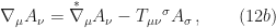
By substituting (9) into the equations (1), the covariant derivative $\nabla$ can be expressed in terms of the Christoffel connection {} and the tensor T, thus:

$\nabla_\mu A^\nu = \partial_\mu A^\nu + (\{\, \overset{\nu}{{}_{\mu\sigma}} \} + T_{\mu\sigma}{}^\nu) A^\sigma \, ,\qquad (10a)$ ,

$\nabla_\mu A_\nu = \partial_\mu A_\nu - (\{\, \overset{\sigma}{{}_{\mu\nu}} \} + T_{\mu\nu}{}^\sigma) A_\sigma \, , \qquad (10b)$

which can be re-grouped as follows:

$\nabla_\mu A^\nu = (\partial_\mu A^\nu + \{\, \overset{\nu}{{}_{\mu\sigma}} \} A^\sigma ) + T_{\mu\sigma}{}^\nu A^\sigma \, , \qquad (11a)$

$\nabla_\mu A_\nu = (\partial_\mu A_\nu - \{\, \overset{\sigma}{{}_{\mu\nu}} \} A_\sigma ) - T_{\mu\nu}{}^\sigma A_\sigma \, .\qquad (11b)$

The terms in the parentheses ( ) on the right-hand sides of Equation (11) are covariant derivatives using the Christoffel connection {}. Denoting a covariant derivative using the Christoffel connection by $\overset{*}{\nabla}$ , the equations (11) can be re-expressed as:

$\nabla_\mu A^\nu = \overset{*}{\nabla}_\mu A^\nu + T_{\mu\sigma}{}^\nu A^\sigma \, ,\qquad (12a)$

$\nabla_\mu A_\nu = \overset{*}{\nabla}_\mu A_\nu - T_{\mu\nu}{}^\sigma A_\sigma \, ,\qquad (12b)$

and the important property that the Christoffel connection is metric can be written:

$\overset{*}{\nabla}_\lambda\, g_{\mu\nu} \overset{\mathrm{def}}{=} \partial_\lambda g_{\mu\nu} - \{\, \overset{\sigma}{{}_{\lambda\mu}} \} g_{\sigma\nu} - \{\, \overset{\sigma}{{}_{\lambda\nu}} \} g_{\mu\sigma} = 0 \qquad\qquad (13)$ .

Symmetry or anti-symmetry in indices is denoted by round or square brackets, respectively, and there is a division by a factor of $n!$ for the n indices involved in the (anti-)symmetrisation. For our purposes, the symmetric and anti-symmetric parts of a general rank-2 tensor $B_{\mu\nu}$ can be denoted

$B_{(\mu\nu)} = \tfrac{1}{2} B_{\mu\nu} + \tfrac{1}{2} B_{\nu\mu}\, ,\qquad (14a)$

$B_{[\mu\nu]} = \tfrac{1}{2} B_{\mu\nu} - \tfrac{1}{2} B_{\nu\mu}\, ,\qquad (14b)$

and any tensor $B_{\mu\nu}$ can always be separated into a symmetric and an anti-symmetric part:

$B_{\mu\nu} = B_{(\mu\nu)} + B_{[\mu\nu]}\, . \qquad (15a)$

It is also possible (Carroll 2004, p129) to split the symmetric part $B_{(\mu\nu)}$ into two further components: the trace $B = g^{\mu\nu}B_{(\mu\nu)}$ , and a trace-free part $\widehat{B}_{\mu\nu} = B_{(\mu\nu)} - \tfrac{1}{n} B g_{\mu\nu}$ , where n is the dimension of the space. For a 4-dimensional space like spacetime, (15a) can be rewritten as

$B_{\mu\nu} = \tfrac{1}{4} B g_{\mu\nu} + \widehat{B}_{\mu\nu} + B_{[\mu\nu]}\, . \qquad (15b)$

These three elements of the tensor B define “invariant subspaces” such that, as Carroll notes, under a change of coordinates “the different pieces are rotated into themselves not into each other” (ibid.). They are, therefore, in a certain sense, quasi-independent pieces of the whole tensor.

This index (anti-)symmetrising process generalises to other tensors having more than two indices. For our purposes later we need only consider (anti-)symmetrisation of no more than three indices. Thus, symmetrising over 3 indices, hence the factor $\tfrac{1}{3!}=\tfrac{1}{6}$ , by taking permutations of the indices, yields

$C_{(\mu\nu\lambda)} = \tfrac{1}{6} ( C_{\mu\nu\lambda} + C_{\lambda\mu\nu} + C_{\nu\lambda\mu} + C_{\mu\lambda\nu} + C_{\lambda\nu\mu} + C_{\nu\mu\lambda})\, , \qquad (16a)$

while the analogous anti-symmetrisation looks like

$C_{[\mu\nu\lambda]} = \tfrac{1}{6} ( C_{\mu\nu\lambda} + C_{\lambda\mu\nu} + C_{\nu\lambda\mu} - C_{\mu\lambda\nu} - C_{\lambda\nu\mu} - C_{\nu\mu\lambda})\, . \qquad (16b)$

This operation is most easily done by first doing a cyclic permutation $(\mu\rightarrow\nu\rightarrow\lambda\rightarrow\mu)$ to generate the first three terms, and then swapping the 2nd and 3rd indices of each of these three terms, to give the second three terms (note how the first index is the same for the 1st and 4th, 2nd and 5th and 3rd and 6th terms). For symmetrisation, all signs are made positive, whereas for anti-symmetrisation, the odd permutations (i.e., the “swapped” indices in the 2nd group of three terms) are all negative, whence, (16b) is easily obtained from (16a) by making each odd (“swapped”) permutation negative.

If any index is excluded from the index mixing, it is separated off by way of vertical bars | |, thus:

$C_{(\mu| \nu | \lambda)} = \tfrac{1}{2} C_{\mu\nu\lambda} + \tfrac{1}{2} C_{\lambda\nu\mu}\, , \qquad (17a)$

and similarly for anti-symmetry,

$C_{[\mu| \nu | \lambda]} = \tfrac{1}{2} C_{\mu\nu\lambda} - \tfrac{1}{2} C_{\lambda\nu\mu}\, , \qquad (17b)$

noting that the factor of division is $\tfrac{1}{2}$ because only 2 indices are being mixed.

OK, so that sets the scene for the next part, where we will examine the geometry of the space of the semi-symmetric metric connection to see what geometrical objects exist there and how these compare to or differ from the objects we are familiar with from the Riemannian space of GR.

Next time: Part III: The Geometry

References

Carroll, SM 2004, Spacetime and geometry: An introduction to general relativity, Addison-Wesley.

Göckeler, M and Schücker, T 1989, Differential geometry, gauge theories, and gravity, Cambridge monographs on mathematical physics, Cambridge University Press.

Infeld, L 1942, Quest: The evolution of a scientist, Readers Union / Victor Gollancz, London.

Pais, A 1982, Subtle is the Lord: The science and life of Albert Einstein, Oxford University Press.

Schouten, JA 1954, Ricci-calculus: An introduction to tensor analysis and its geometrical applications, 2nd edn, Springer-Verlag, Berlin.

Main image: Cartoon in The Washington Post 19 April 1955 by Herb Block (detail).

Mathematical Preliminaries

References

Share this:

Leave a comment Cancel reply