
The Background
Many years ago (getting close to 30 now), while doing my PhD (Voros 1996) in theoretical physics on mathematical extensions to General Relativity – and in particular, on Einstein’s own “unified field theory” – I happened across a book by Jan Schouten (1954) called Ricci-Calculus, which was an introduction (by a mathematician) to tensors and their applications, especially to geometrical thinking and analysis.
Now, if you know General Relativity (hereafter “GR”) – which is Einstein’s theory of gravitation – then you’ll know that Einstein worked with geometrical objects called “tensors” (or more precisely, tensor fields) to formulate the field equations of GR using “tensor analysis” or “tensor calculus”. (“What’s a tensor,” you ask? Well, a tensor is a bit like a vector, only more so. 🙂 In actual fact, a vector is a particular type of tensor, but this is not the place for more detailed definitions.)
This formulation was done principally in what is known as the “component” (notation) form of tensor analysis, which uses symbolic representations of the component functions that describe an object, rather than a more geometrically-oriented abstract representation of the object itself. (This latter is much more common these days, and mathematicians tend to prefer to stick to the elegant component-free representation for the most part. Physicists, on the other hand, tend to work more directly with the component notation, mostly for pragmatic reasons, given that they are usually wanting to carry out calculations, which generally requires accessing individual components.)
\begin{brief explanatory aside}
For example, an ordinary 3-vector (i.e., a vector in 3-dimensional space) is often written simply as a boldface letter v, which emphasises its “geometric object” aspect. But, when we are instead looking at the vector’s components along the x, y and z directions, it is often written something like this:
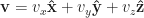
where the “hat” forms 


The three basis vectors 


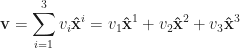
where the 


which saves a bit of writing (although the index placements – i.e., up or down – can change in more general spaces than the 3-D space with which we are familiar).
\end{brief explanatory aside}
So, to the matter at hand.
As we will see later, the geometrical space that is used as the basis for GR (“Riemannian” or sometimes just “Riemann” geometry) has a special set of assumptions about the nature of some important objects defined in the geometrical space, mostly to do with certain types of “symmetry” they possess. Now, as I was working on mathematical extensions to GR – and in particular Einstein’s own non-symmetric unified field theory (although I also looked at a few others along the way) – you might get an intuitive sense right away that because of its “non-symmetric” nature it was going to be even more complicated than anything found in (symmetric) GR (which, we’ll see, is complicated enough!). And indeed it was, both in terms of the underlying geometry, as well as in terms of the field equations for the two fields Einstein was attempting to unify, these being gravitation (which is what GR is a theory of, as mentioned) as well as electromagnetism.
We will see later that the geometrical space of GR, Riemannian geometry, can be derived from two key assumptions concerning two fundamental objects found in certain geometrical spaces – the metric tensor, usually denoted by 

In general, the metric of a geometrical space is a “symmetric” tensor, which can be represented – for a four-dimensional space – by a symmetric 
The connection, by contrast, is not a tensor, and does not necessarily possess any sort of “symmetry”, so it can in general be “non-symmetric”. However, any general non-symmetric connection can always be uniquely decomposed into the sum of a symmetric part which is not a tensor, and an anti-symmetric part which is a tensor, which latter is generally known as the “torsion” tensor (the anti-symmetry introduces a kind of “twisting” into the connection, hence its name).
The important assumptions underlying the Riemannian geometry of GR are that if, in a general space, the connection is assumed to be (i) symmetric (and thereby having no torsion), and (ii) metrical or metric (sometimes metric compatible), which means that the covariant derivative of the metric tensor with respect to that connection vanishes (i.e., = 0), then one recovers uniquely the underlying Riemannian geometry of GR, as well as the extremely important relationship which defines the connection wholly in terms of functions of the metric – the so-called “Christoffel symbol” or Christoffel connection, which we might therefore characterise as the (unique) symmetric metric connection.
This relationship between metric and connection ends up making every important tensor in the space – including the tensor known as the curvature (or Riemann) tensor – ultimately a function of the metric. It is in this way that Einstein’s theory of gravitation is a pure geometrical theory of gravity, because a curvature tensor wholly expressible in terms of the metric produces a geometrical space whose “shape” is, as it were, “doubly” defined by way of the metric, while the field equations of GR are ultimately equations for the metric via the curvature as it relates to and is influenced by the distribution of matter-energy in spacetime. In other words, in GR, the mathematical geometrical “space” (Riemannian geometry) is assumed to represent actual spacetime itself – quite successfully, as it turns out, since it has been fully verified in every experimental test it has ever been subjected to for the last century (although see later in this series of posts for some further comments about this).
Pre-empting things a little bit (I’ll go into more detail in later posts), Einstein’s original field equations of 1915 can be written in the form:

where 

Now, my PhD work was on a non-symmetric generalisation of GR undertaken by Einstein himself, begun about a decade after GR was published. Einstein’s unified field theory (hereafter “EUFT”) dropped the assumptions of symmetry of the underlying space in an attempt to see if electromagnetism could also be incorporated into such an expanded non-symmetric geometrical theory. The search for such a unified field theory was prompted in Einstein’s mind by the (to him quite unsatisfactory) separation of geometric field and mass-energy in Equation (1). He said of it (writing in Schilpp 1949, p.75):
The right hand side is a formal condensation of all things whose comprehension in the sense of a field-theory is still problematic. Not for a moment, of course, did I doubt that [the] formulation [
And (Einstein 1954, p.311):
It is sufficient – as far as we know – for the representation of the observed facts of celestial mechanics. But it is similar to a building, one wing of which is made of marble (left part of equation), but the other wing is made of low grade wood (right part of equation). The phenomenological representation of matter is, in fact, only a crude substitute for a representation which would do justice to all known properties of matter.
As I noted in my PhD thesis (1996, chap. 2, sect. 2):
It was this “crude”-ness which prompted Einstein’s further work toward a unified field theory – a theory where there would be pure field equations with no explicit sources. In other words, EUFT was motivated by the desire to get rid of the
It is widely held that he did not succeed in this quest (indeed, this is now folklore in physics – and many people have written about and sometimes lamented that he spent his final years on such a “fruitless” search…). However, my doctoral work demonstrated that the two main published analyses of the electrodynamics of EUFT – which allegedly showed that EUFT does not produce the correct equations of motion for charged particles and so must therefore be physically unviable – are actually inconclusive as a test of the viability of EUFT; so, therefore, it argues, one cannot conclude, on the basis of those analyses, that the theory is indeed unviable. Of course, this statement is quite different from saying the theory does work. It’s just that one cannot say anything, one way or the other about the viability of EUFT on the basis of those earlier analyses, and so – since it was rejected on the basis of those analyses – it was actually rejected for the wrong reason. This result was written up for a journal article, eventually published in 1995 (Voros 1995).
During the time that I was trying to work out the electrodynamical terms implied by a suitably-refined analysis of the electrodynamics of EUFT, I was delayed for several months while awaiting a copy of a PhD thesis from the University of Toronto. That thesis (Wallace 1940) contained the details of how to derive the equations of motion for charged particles when Maxwell’s electromagnetic theory is added to GR by making the
Very early in my candidature, I had found the aforementioned book by Schouten in the University’s library, which I was reading to try to understand more fully the various properties of non-Riemannian geometrical spaces – including the space of EUFT – and the various important tensors which can be defined within them in the general case beyond the special assumptions of the Riemannian geometry of GR. Internal disputes at UT led to a delay in getting hold of Wallace’s work, and it was due to this delay that, for something useful to do while I waited, I went back to Schouten’s book and continued exploring a most beguiling idea I had come across there earlier, during my preparatory research into general geometrical spaces – an idea which I’ll describe below.
As noted above, the Christoffel connection is the unique connection which emerges from assuming a (symmetric) metric tensor and a torsion-free (i.e., symmetric) connection, while simultaneously assuming that the connection is also metrical/metric (i.e., the covariant derivative of the metric with respect to that connection vanishes) – to wit: the symmetric metric connection. Schouten noted his results as part of a wide-ranging and magisterial discussion of the properties of general geometrical spaces, and then very elegantly derived specific cases resulting from particular assumptions to show how these special cases arise as a result of those assumptions.
One of the consequences for EUFT, arising from the relaxation of the simplifying assumptions of symmetry found in GR, was its incredible complexity, both in terms of the underlying geometry as well as the field equations – I used to (only half-jokingly) say that 
In electromagnetic theory, the electromagnetic field is often represented by an anti-symmetric tensor, conventionally written 
But, the electromagnetic field can also be represented by a 4-vector potential 
Now enter a discussion from Shouten, chapter III, section 2, which introduces a type of connection called semi-symmetric for which the skew part (i.e., the torsion) has the most interesting form (which is clearly anti-symmetric in the indices 


where 


which can be visualised as a 
In other words, a semi-symmetric connection seems to introduce a single 4-vector field into the connection! This is very interesting! And, furthermore, in Section 4 of the same chapter (on p.142), it is observed that there is a unique, “metric semi-symmetric connection”, which adds to the usual Christoffel connection of Riemannian geometry an extra term of the form

Wow! If ever there was a candidate for a minimalist extension of GR which introduces only a single 4-vector field, then this has got to be it! I called it the MSSC (“metrical semi-symmetric connection”) for a long time (indeed my main notebook and the sundry loose notes all use this shorthand term), but I have since recently found that mathematicians working on this topic tend to refer to it as the semi-symmetric metric connection, so I have now changed the way I refer to it in order to reflect this.
Hence, the upcoming series of posts, of which this one is marked as the first. The intention is to describe the work I did on the semi-symmetric metric connection (SSMC) as a possible extension to the (Riemannian) geometry of GR, which was done in order to see whether it might be able to model the addition of the electromagnetic field to GR in a geometrically-unified way, given that the SSMC adds only a single new object to Riemann geometry – to wit, an object of precisely a most very-highly suggestive form, namely, a 4-vector.
I spent a fair bit of time trying to nut this idea out over the years, starting about 1989/1990 or so when I first saw the SSMC in my preliminary reading of Schouten, and more subsequently to that. But each time I have had to put it aside – not the least of which reason in those days was to actually finish the PhD on the topic I had started with – the electrodynamics of EUFT – and definitely once the Wallace thesis showed up and I could get on with the electromagnetic calculations for EUFT. Following completion, of course, there was paid work to find, then marriage, etc, and life beyond the comparative haven (I now realise) of postgraduate study ramped up considerably – and had practically nothing to do with physics anymore – so the SSMC exploration project has waxed and waned over the years (mostly waned). Another reason I put it aside back then was that I soon found a paper in General Relativity and Gravitation – or maybe it was in Classical and Quantum Gravity – which had already done pretty much the same thing a couple of years earlier, namely added a vector field to the Christoffel connection such that the covariant derivative was metrical, and the SSMC dropped out, but I don’t think the author called it that. If I recall correctly (nearly 30 years later!), I think he used a Lagrangian formulation to derive field equations, the details of which implied a massive vector field, as opposed to a massless one, which is what the EM field is assumed to be. Therefore, I felt that using a Lagrangian approach to finding field equations for the SSMC was not going to work for electromagnetism – it seemed to me that some other way was needed, combined with a very careful comparison with what GR becomes when electromagnetism is added (the so-named Einstein-Maxwell Theory), and how far one can push the analogy, given that EMT has not been tested experimentally (only the free-space field equations of GR have ever been tested).
But, every few years I have tended to go back to my notes – the earliest ones were from around 1990 or so (now lost), and I copied some of the later loose notes into a workbook in early 1998 to ensure they didn’t get lost, too) – or sometimes directly to Schouten’s book itself, and try once again to derive plausible field equations implied by this form of connection, using arguments based in physics (and not from a Lagrangian), much as Einstein had done for the field equations of GR arising from results in Riemannian geometry. But, I have never quite got there… It always feels like I get close, but my ability to shuffle tensors and tensor indices around is very oxidised these days, compared to 30 years ago, so it always seems as though there is some clever trick or an important insight that is dangling just beyond the reach of my increasingly-addled, and now quite middle-aged, brain …
Nonetheless, I hope that by making these explorations public and open – and having to clarify and explain to others what I had tried to do all those years ago (and since) – it might lead to someone else examining these ideas and might possibly nudge them to have a try, and yield a coherent mathematical theory which, one hopes, could be tested – both for internal consistency and for empirical validity. A poster that was attached to the wall above my desk when I was a PhD student was a quote from 1969 Nobel Laureate Murray Gell-Mann. In an interview for Omni magazine in 1985 he noted (Schultz 1985, p.94):
In theoretical physics we use very simple tools: pencil and paper, eraser, chair and table. More important than any of these is the wastebasket. Almost every idea that occurs to a theoretical physicist is wrong. And it can be wrong on various grounds. The simplest grounds for being wrong have to do with logical inconsistencies. Once the idea or theory is logically consistent, there is also the question of whether it agrees with a system of well-established observations. The theory has to agree with itself, and it has to agree with nature. Those are the requirements, and most theoretical ideas don’t meet them. So we crumple up most of our pages of scribbles and throw them away.
When, after many a long session of scribbling tensor equations in the various theories I was looking at, it turned out that some calculation or other yielded either no result or landed in a dead-end from which no return was possible, I would – as Gell-Mann said – have to crumple up those pages of scribbles. Then, while hurling them towards the nearest wastebasket or recycling bin – and to the frequent consternation of my fellow students in our shared office – I would very often say out loud and with no small amount of exasperation: “and here’s another one for you, Murray!” 😉 Then, it would be time for more coffee, and a sanity break, before starting it up all over again… 🙂 Over the years people have asked me what it was like to do theoretical physics. The only sensible explanation I’ve ever been able to come up with is this: Listen to the second movement of Beethoven’s Ninth Symphony. For me, it’s like that.
So, that’s the background – how and why the SSMC came to be lodged in my mind 30-odd years ago. It has hung around on the backburner ever since, occasionally popping up for a brief visit, sometimes even being treated to a more extended stay for a bit of tensor-fun-and-games every few years. But, overall, I feel that I had pretty much stalled on the exploration of this quite lovely and elegantly simple idea. So, I am undertaking this series of blog posts with the intention of them hopefully triggering new sets of eyes to see if, just maybe, the SSMC could be the basis of a “minimalist” classical geometrically-unified theory of gravity and electromagnetism – the two “macroscopic” fields – based on extending GR. Even a “limited” unified theory of just these two macroscopic fields (as opposed to the full-blown complete unified field theory of everything which is the current Holy Grail of physics) would still be an interesting thing to have.
Of course, there have been attempts to add torsion to GR before (e.g., “Einstein-Cartan theory”) but these have tended to involve non-symmetric energy-momentum tensors and attempting to model “spin” (a property of quantum particles). I did not go down that line because I was interested in how far SSMC geometry could be pushed vis á vis classical electromagnetism. I also wanted to avoid the use of a Lagrangian variational procedure to derive the field equations, for the reason stated above, preferring rather to use arguments and ideas from physics to do so, just as Einstein did for GR. More on that later.
Sometimes, the process of explaining something to someone else causes unexpected connections and produces insights that a silent internal conversation with oneself will never yield.
Therefore, let’s see how it goes, this time around …
Next time: Part II: Mathematical preliminaries
References
Einstein, A 1954, Ideas and opinions, Bonanza Books, New York. Based on Mein Weltbild edited by Carl Seeling, and other sources. New translations and revisions by Sonja Bargmann.
Schilpp, PA (ed.) 1949, Albert Einstein: Philosopher-scientist, vol. 1, Harper and Row, New York.
Schouten, JA 1954, Ricci-calculus: An introduction to tensor analysis and its geometrical applications, 2nd edn, Springer-Verlag, Berlin.
Schultz, R 1985, ‘Interview: Murray Gell-Mann’, Omni, vol. 7, no. 8, May, pp. 54-58, 92-94.
Voros, J 1995, ‘Physical consequences of the interpretation of the skew part of
Voros, J 1996, On the electrodynamics of Einstein’s non-symmetric unified field theory, PhD thesis, Dept of Physics, Monash University, Melbourne, Australia. (Australian) National Bibliographic Database (ANBD) Record number 12976078. https://nla.gov.au/anbd.bib-an12976078. A version typeset as a normal-sized, two-sided book is available as a PDF from both Academia.edu and ResearchGate.
Wallace, PR 1940, On the relativistic equations of motion in electromagnetic theory, PhD thesis, Dept of Mathematics, University of Toronto, Toronto, Canada.
Main Image – the title section of the 1915 paper describing General Relativity: “The Field Equations of Gravitation”. Image Credit: John D Norton, University of Pittsburgh. https://www.pitt.edu/~jdnorton/teaching/HPS_0410/chapters/general_relativity_pathway/index.html

What’s EUFT?
Also, how do I put the contents of my exploded brain back?
Tracey Tritsch LongDog & Associates m: 0414 555 616 e: tracey@longdog.com.au w: http://www.longdog.com.au w: au.linkedin.com/in/traceytritsch t: @traceytritsch
>
LikeLike